Navigation
Sidebar
Table of Contents
Get Started
WebPower consists of a set of calculators for a variety of power analyses. It also provides the path diagram based interface for more general and advanced power analyses. We use a few example to illustrate the use of WebPower here. More details can be found in the manual of WebPower.
Example 1. Calculate power for correlation
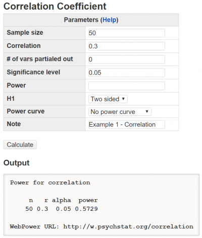
A student wants to study the relationship between stress and health. Based on her prior knowledge, she expects the two variables to be correlated with a correlation coefficient of 0.3. If she plans to collect data from 50 participants and measure their stress and health, what is the power for her to obtain a significant correlation using such a sample?
The input and output for calculating power for this study are given in the figure below. In the field of Sample size, input 50, the total number of participants; and in the field of Correlation, input 0.5, the expected effect size. The number of variables partialed out is 0. The default significant level 0.05 is used although one can change it to a different value. The field for Power is left blank because it will be calculated. The H1 is “two sided” corresponding to the null hypothesis that the correlation is 0 and the alternative hypothesis that the correlation is not 0. A simple note “Example 1 - Correlation” is also added in the Note field. By clicking the “Calculate” button, the statistical power is given in the output immediately. For the current design, the power is 0.573.
Example 2. Power curve for t-test
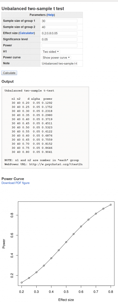
There are two groups of students. Students in group A use learning strategy A and students in group B use learning strategy B. One researcher plans to recruit 30 students for group A and 40 students for group B. If the researcher does not know the effect size but expects the effect size to be in the range from 0.2 to 0.8, the researcher can obtain a power curve with each potential effect size value.
Figure below shows the input and output for a study with 30 participants in group A and 40 participants in group B. Note that in the Effect size field, the input is 0.2:0.8:0.05, which includes a sequence of effect sizes from 0.2 to 0.8 with the interval 0.05. In the output, the power for each effect size is listed. The power curve is displayed at the bottom of the output. The power curve can be used for interpolation. For example, to get a power at least 0.8, the effect size should be somewhere between 0.65 and 0.7.
Example 3. Sample size planning for regression
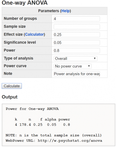
A student hypothesizes that freshman, sophomore, junior and senior college students have different attitude towards obtaining arts degrees. Based on his prior knowledge, he expects that the effect size is about 0.25. Suppose the student wants to know the sample size needed to get a power 0.8. In this situation, the Sample size field is left blank while in the Power field, the value 0.8 is the input. In the output, we can see a sample size 179 is needed to obtain a power 0.8, that is about 45 for each group.
Example 4. Power for SEM
Satorra and Sarris (1985) presented an example in which $Y_{1},Y_{2},Y_{3},Y_{4}$, and $X$ satisfy the following population model $$ \begin{eqnarray} Y_{1} & = & \gamma_{1}X+\zeta_{1}\nonumber \\ Y_{2} & = & \gamma_{2}X+\beta_{21}Y_{1}+\zeta_{2}\label{eq:sem-chisq-full}\\ Y_{3} & = & \gamma_{3}X+\zeta_{3}\nonumber \\ Y_{4} & = & \beta_{41}Y_{1}+\beta_{42}Y_{2}+\beta_{43}Y_{3}+\zeta_{4}\nonumber \end{eqnarray} $$ where $\zeta_{i},i=1,2,3,4$ follows a normal distribution with mean 0 and unknown variance $\psi_{i}$, and $X$ has mean 0 and variance 1. The parameter values are
| Parameter | $\gamma_{1}$ | $\gamma_{2}$ | $\gamma_{3}$ | $\beta_{41}$ | $\beta_{42}$ | $\beta_{43}$ | $\beta_{21}$ | $\psi_{1}$ | $\psi_{2}$ | $\psi_{3}$ | $\psi_{4}$ |
|---|---|---|---|---|---|---|---|---|---|---|---|
| value | .4 | .5 | .4 | .4 | .4 | .4 | .2 | .84 | .61 | .84 | .27 |
Suppose a model is fitted without $\beta_{21}$. Then, one can investigate the power to detect the path $\beta_{21}$ using the likelihood ratio test.
Effect size calculation
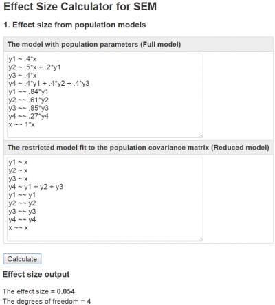
To conduct the power analysis, we first determine the effect size. For many applications, we have included the effect size calculator. For example, for the SEM analysis, the following input obtains the effect size 0.054.
Power analysis
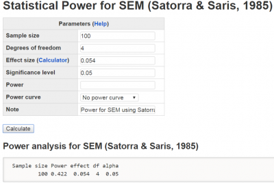
A researcher is interested in the power given she can collect data from 100 participants. The input and output for calculating power for this study is given in Figure below. In the Sample size field, we input 100 and in the Degrees of freedom field, we input 4. The Effect size is 0.054. The default Significance level 0.05 is used. The field for Power is left blank because it will be calculated. By clicking the “Calculate” button, the statistical power is given in the output immediately. For the current analysis, the power is 0.422.
Example 5. Minimum detectable effect size for SEM
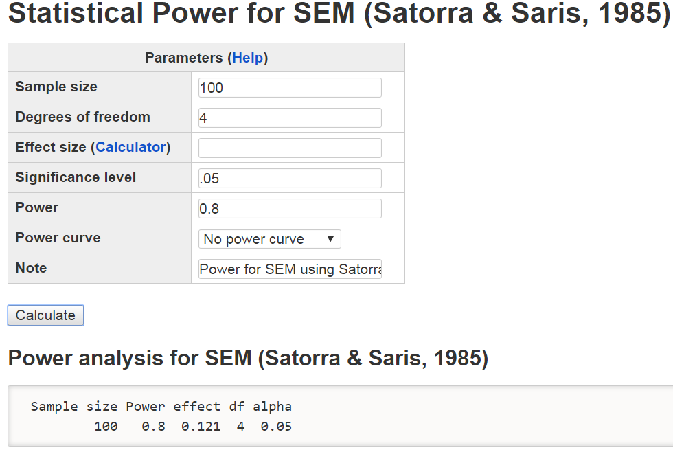
Suppose a researcher does not have enough information to determine the size of effect. In this case, the researcher can detect the minimum effect to achieve certain power given the sample size. Such an effect can help the researcher determine whether it is meaningful to conduct a study. For example, if an unreasonably large effect is needed, it might be difficult to achieve significant results. In Figure below, we calculate the effect size by proving both sample size and power as well as other information. Note that the effect size has to be at least 0.121 to have a power 0.8 with the sample size 100.
Examples on the use of path diagrams
Example 1. Mediation analysis
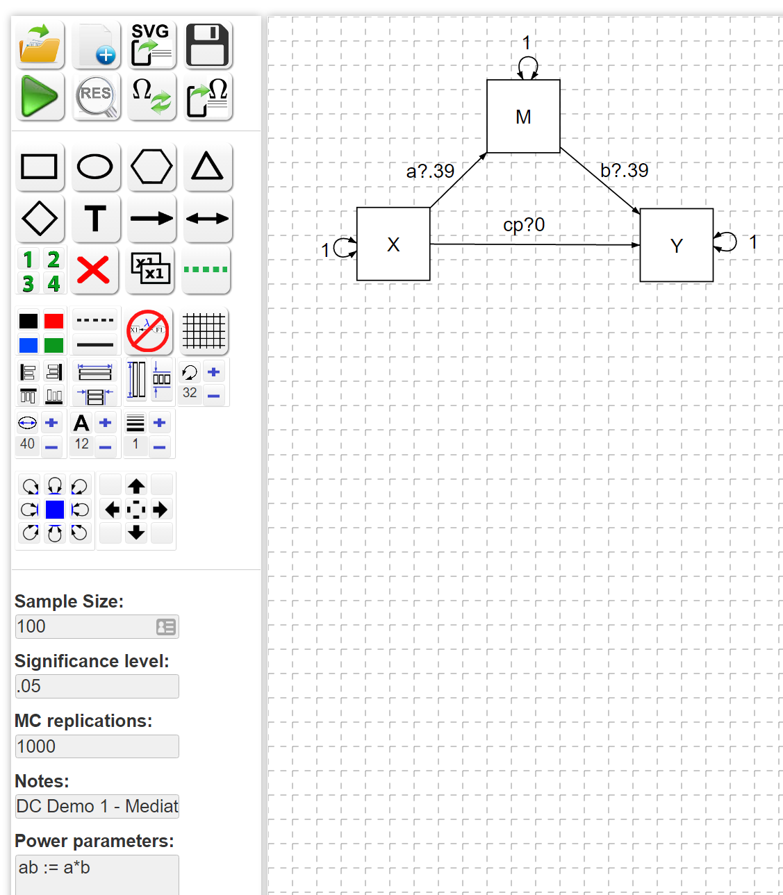
Draw a path diagram as shown below
The output is given below
Please refresh your browser if you are expecting more output.
Basic information:

  Esimation method                                  ML
  Standard error                              standard
  Number of requested replications                1000
  Number of successful replications               1000
  Sample size

                       True  Estimate      MSE      SD     Power Power.se Coverage
Regressions:
  M ~
    X         (a)      0.390    0.387    0.100    0.100    0.970    0.005    0.951
  Y ~
    M         (b)      0.390    0.389    0.100    0.105    0.968    0.006    0.935
    X        (cp)      0.000    0.002    0.107    0.110    0.057    0.007    0.943

Intercepts:
    M                  0.000    0.001    0.099    0.102    0.057    0.007    0.943
    Y                  0.000    0.003    0.099    0.104    0.072    0.008    0.928
    X                  0.000   -0.004    0.100    0.101    0.052    0.007    0.948

Variances:
    M                  1.000    0.980    0.139    0.140    1.000    0.000    0.926
    Y                  1.000    0.971    0.137    0.139    1.000    0.000    0.914
    X                  1.000    0.999    0.141    0.144    1.000    0.000    0.940

Indirect/Mediation effects:
    ab                 0.152    0.150    0.056    0.055    0.870    0.011    0.933
WebPower ended at 16:09:41 on Dec 09, 2016
Time spent on the analysis
   user  system elapsed
137.005   0.505 137.513

