Navigation
Sidebar
Table of Contents
Power of t test
Description
Power calculation / sample size planning based on t test. Works for one-sample t test, paired two-sample t test, and two-sample t test with equal group sizes. It uses the R function power.t.test for power calculation.
Arguments
Among sample size, True difference, sd, significance level, and power, one and only one can be left blank.
Sample Size
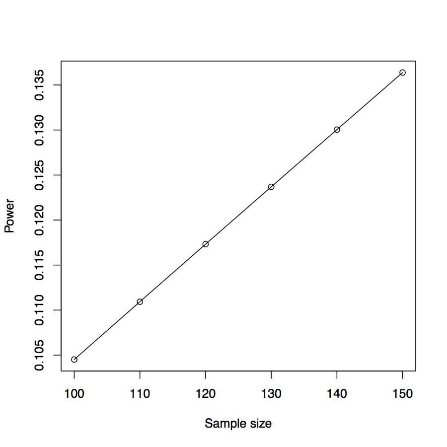
Provide the number of observations per group. Multiple sample sizes can be provided in two ways. First, multiple sample sizes can be supplied separated by white spaces, e.g., 100 150 200 will calculate power for the three sample sizes. A sequence of sample sizes can be generated using the method s:e:i with s denoting the starting sample size, e as ending sample size, and i as the interval. For example, 100:150:10 will generate a sequence 100 110 120 130 140 150.
By default, the sample size is 100.
Effect Size
The effect size can be calculated based on the effect size calculator.
The effect size to be used. Multiple effect sizes or a sequence of effect sizes can be supplied using the same method for sample size.
By default, the value is 0.1.
Significance Level (alpha)
The significance level (Type I error rate) for power calculation withe the default 0.05.
Power
The power of the test.
Type of test
One- two- or paired-samples.
H1
Specifying the alternative hypothesis, can be “two.sided” (default), “greater” or “less”
Power curve
Whether to generate the power curve.
Note
A note (less than 200 characters) can be provided to provide basic information on the analysis.
Output
The output lists the related information about this power analysis. The output is given as a matrix.
   n Difference sd alpha Power
 100       0.10  1  0.05  0.10
An example of power curve

